NOTE: This article, “Decoding Mathematical Notation: A Guide to Understanding Optimization Problems in Human Language,” is part of the “Optimization with Python and Pyomo: A Comprehensive Tutorial Series” – your go-to resource for mastering optimization techniques.
Hey there, optimization enthusiasts! In today’s blog post, titled “Decoding Mathematical Notation,” I want to share some insights on how to read and understand mathematical notation when formulating optimization problems. I remember back in my bachelor’s and master’s days, many of my friends (including myself, of course) felt nervous when faced with optimization problems in the form of mathematical programming. One reason for this was the seemingly complex mathematical notation used throughout. For instance, you’ll find plenty of intricate mathematical notations like these in textbooks on mathematical programming and optimization:

Encountering mathematical notation like this can certainly cause panic for those who aren’t used to practicing and understanding the meaning behind it. Back in college, I remember trying to read it over and over again until I finally grasped its meaning. It felt like I was a human trying to decipher an alien language, haha!
In this blog post, I’ll attempt to explain some fundamental mathematical notations essential to mathematical programming, and most importantly, how to interpret them in human language!
a. List of fundamental notations and their interpretations
- Objective function:
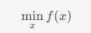
This notation means we want to minimize the function f(x) with respect to x. In other words, we want to find the value of x that results in the lowest possible value for the function f(x).
- Constraints:

This notation represents a set of constraints on the variables x, where each constraint is represented by a function g_i(x) that must be less than or equal to some constant b_i. There are m constraints in total, and each one is indexed by i.
- Equality constraints:

This notation represents a set of equality constraints on the variables x, where each constraint is represented by a function h_j(x) that must be equal to some constant c_j. There are p constraints in total, and each one is indexed by j.
- Bounds on variables:
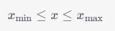
This notation means that the variables x must be within a certain range, with a lower bound of x_min and an upper bound of x_max.
- Summation:

This notation means to sum up all the terms a_i, where i starts at 1 and goes up to n. It is often used to represent the sum of all elements in a set or the sum of all terms in a sequence.
- Product:

This notation means to multiply all the terms a_i, where i starts at 1 and goes up to n. It is often used to represent the product of all elements in a set or the product of all terms in a sequence.
To start, I believe it’s crucial to understand the meaning of at least these six notations. Familiarizing myself with reading and interpreting these notations has been incredibly helpful in tackling more complex optimization problems and formulations. In the following sections, I’ll try to break down these mathematical notations when used to formulate real-world problems, and explain how to read them in everyday language.
b. Examples of optimization problems with their mathematical notations
Now, I’ll attempt to provide some examples of mathematical notation used to formulate real-world optimization problems. To keep this discussion concise and straightforward, I’ll limit the examples to linear programming problems.
- Linear programming – Diet problem
A person wants to create a diet plan with different food items to minimize the total cost while meeting their daily nutritional requirements. The cost of each food item is given, as well as the amount of each nutrient contained in the food item.
Mathematical notation:

Human language interpretation:
Minimize the total cost, which is the sum of the cost of each food item multiplied by the amount of the food item consumed. The total amount of each nutrient must be greater than or equal to the required amount of that nutrient, and the amount of each food item consumed must be non-negative.
- Linear programming – Cargo transport
A company wants to transport goods from several warehouses to multiple customers while minimizing the total transportation cost. The supply capacity of each warehouse and the demand of each customer are given, as well as the transportation cost between each warehouse and customer pair.
Mathematical notation:

Human language interpretation:
Minimize the total transportation cost, which is the sum of the transportation cost between each warehouse (i) and customer (j) pair, multiplied by the amount of goods transported (x_ij). The total amount of goods transported from each warehouse must not exceed its supply capacity (s_i). The total amount of goods received by each customer must be greater than or equal to its demand (d_j). The amount of goods transported between each warehouse and customer pair must be non-negative.
Here, the “for all” symbol (∀) is implicitly used in the constraints. The constraints apply to all warehouses (i) and customers (j). In mathematical notation, we can write it as:

The “for all” symbol (∀) emphasizes that the constraints apply to every warehouse i and every customer j in their respective sets.
- Linear programming – Vehicle Routing Problem (VRP)
I will show you another linear programming example in the transportation domain, focusing on a Vehicle Routing Problem (VRP) with capacity constraints. A delivery company has a fleet of vehicles, and each vehicle has a limited capacity. The company wants to design routes for each vehicle to service a set of customers, starting and ending at a depot, while minimizing the total distance traveled and not exceeding the capacity of each vehicle.
Mathematical notation:

Human language interpretation:
Minimize the total distance traveled, which is the sum of the distance between each pair of locations (i and j), multiplied by a binary decision variable (x_ij) that indicates if the route between locations i and j is used. Each customer must be visited by exactly one vehicle, and each vehicle must leave from and return to the depot (depot is represented by index 0). The total demand of the customers serviced by a single vehicle (represented by q_j for each customer j) must not exceed the vehicle’s capacity (Q). The decision variable x_ij is either 0 (the route is not used) or 1 (the route is used).
In this example, the index i and j include the depot (represented by 0) and the customers (represented by 1 through n). The depot is considered as the starting and ending point for each route.
To help you visualize the VRP, I’ve created a simple graphic representing a transportation network consisting of 1 depot, 10 cities, and a company with 3 truck fleets they want to dispatch. The notation mentioned earlier actually describes a problem like the one depicted below:


That wraps up my blog post on how to read mathematical notation for optimization problems. I hope this article has been helpful and serves as a valuable reference to improve our communication skills using mathematical notation. Thank you for joining me, and I look forward to sharing more insights in future blog posts!



Leave a Comment